Helpful when you are making spreadsheets
Gridlines in Microsoft Excel make it easier to view your data. However, you can disable these gridlines if you don’t want to use them while making spreadsheets. There are multiple ways to remove gridlines in Excel.
You can hide them, fill them with white to make them disappear into the page, or create a template that uses no gridlines.
Quickly Remove Gridlines in Excel
Microsoft Excel has an option that defines whether or not gridlines appear in your spreadsheets. You can disable this option to hide gridlines in your Excel spreadsheets.
This method works on a per-worksheet basis, which means you’ll have to perform these steps for each worksheet to remove gridlines.
- Open your spreadsheet with Microsoft Excel on your Windows or Mac computer.
- Select the worksheet you want to remove gridlines from at the bottom of the spreadsheet.
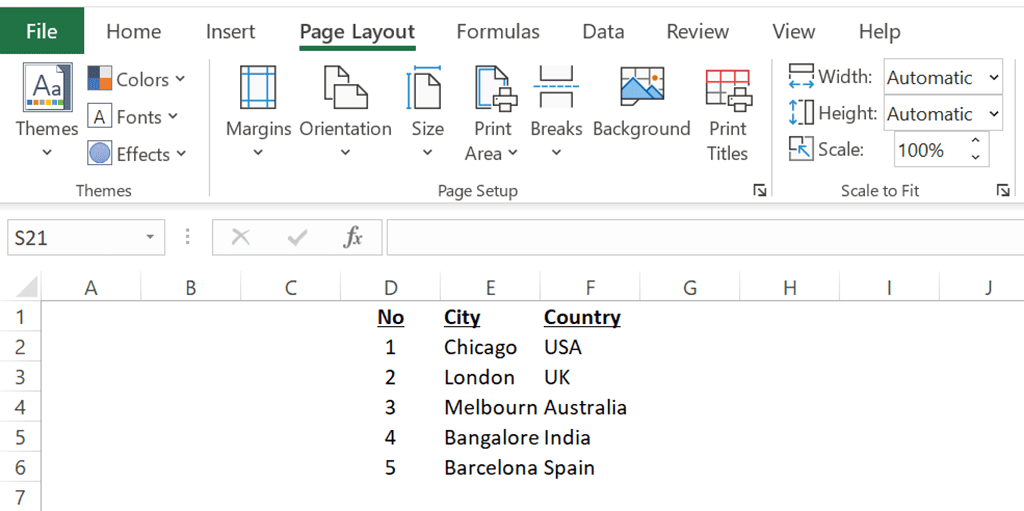
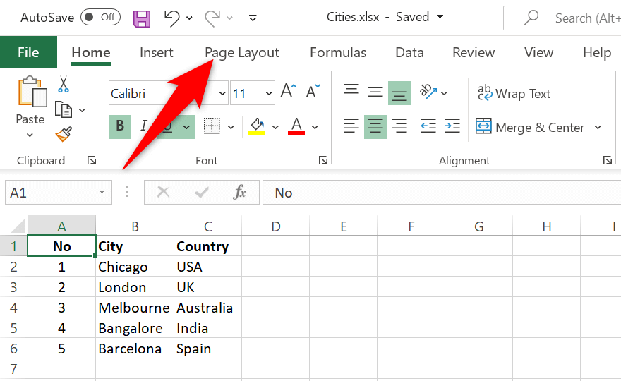
- Select the Page Layout tab at the top of the Excel interface.
- Deselect the View box in the Gridlines section.
Immediately, Excel will hide all gridlines in your current worksheet. If you’d like to bring gridlines back, enable the View box in the Gridlines section.
Change the Gridline Color to Remove Gridlines in Excel
Another way to remove gridlines from an Excel worksheet is by changing the gridlines’ color. By default, Excel uses the grey color for gridlines. If you change this to white, your gridlines will automatically disappear.
Again, this option works on a per-worksheet basis, which means you’ll have to follow these steps for each of your worksheets to remove gridlines.
- Launch your spreadsheet with Microsoft Excel.
- Select the worksheet you want to remove gridlines from.
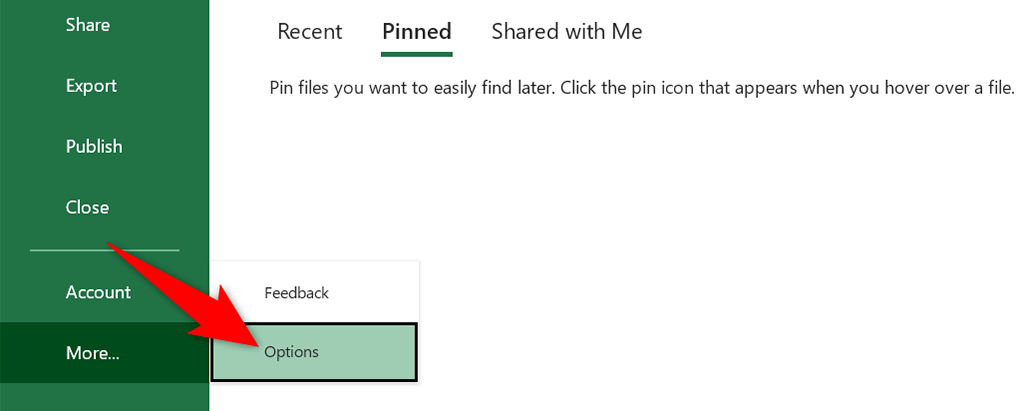
- Select File at the top-left corner of Excel and then choose More > Options from the left sidebar.
- Choose Advanced from the left sidebar on the Excel Options window.
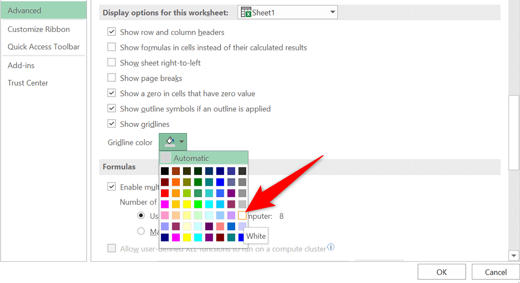
- Scroll down the right pane to the Display options for this worksheet section. Here, select the Gridline color option.
- Choose White in the color list.
- Select OK at the bottom of the window.
All gridlines should now be hidden in your current worksheet.
Apply a Fill Color to Remove Gridlines in Excel
You can fill the white color in your worksheet to make gridlines disappear. Later, if you change your mind, you can remove the fill color to get gridlines back.
- Open the worksheet you want to remove gridlines from.
- Select the cells you want to remove gridlines from. To remove gridlines from your entire worksheet, press Ctrl + A (Windows) or Command + A (Mac) to select your entire worksheet.
- Select the Home tab at the top of the Excel interface.
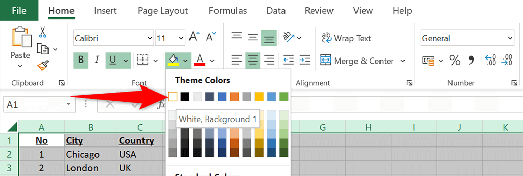
- Select the small down-arrow icon next to the bucket icon and choose the White color.
- Gridlines should now be removed from your worksheet.
To bring gridlines back, choose No Fill from the bucket icon menu.
Remove Gridlines From Specific Rows or Columns in Excel
If you’re looking to remove gridlines from specific rows or columns, use Excel’s Border option. This option allows you to remove gridlines from the selected area in your spreadsheet.
- Open the worksheet you want to hide gridlines in.
- Select the row or the column you want to remove gridlines from.
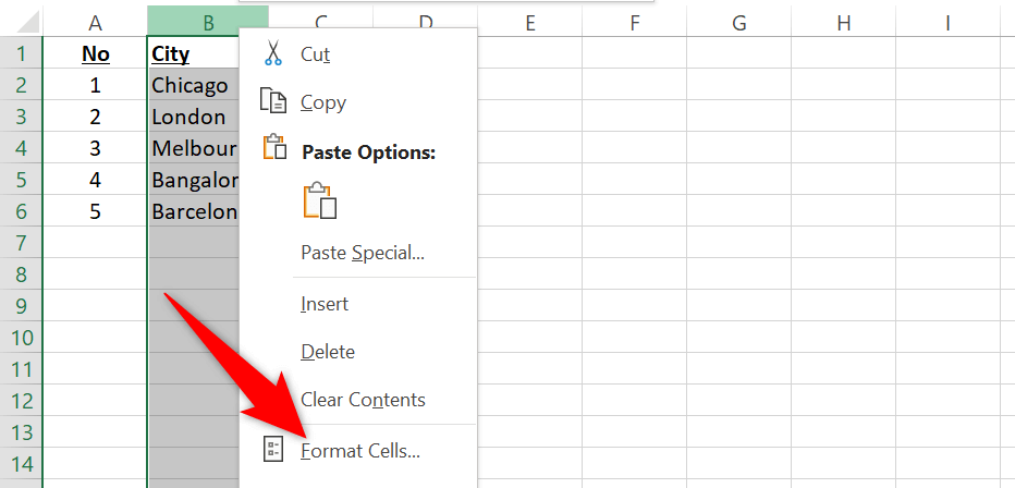
- Right-click the selected column or row and choose Format Cells from the menu.
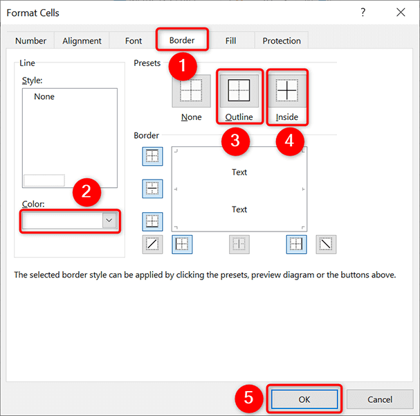
- Select the Borders tab on the Format Cells window. Then, select the Color option and choose the White color.
- Choose Outline and then Inside in the Presets section. Then, select OK at the bottom.
Back on the worksheet screen, you’ll find gridlines from your selected area are now gone.
Always Keep Gridlines Removed in Excel
If you want to make your future spreadsheets without gridlines, create an Excel template that uses no gridlines by default. Then, any spreadsheets that you base on this template will have no gridlines.
To make this template:
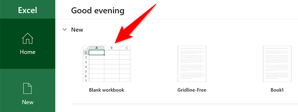
- Open Excel and select Blank workbook to create a new workbook.
- On the editing screen, select the Page Layout tab at the top.
- Deselect the View option in the Gridlines section. This’ll disable gridlines in your current worksheet.
- Save your workbook as an Excel template by selecting File > Save As.
- Choose Excel Template from the Excel Workbook dropdown menu.
- Enter a name for your template (something like Gridline Free) and select Save.
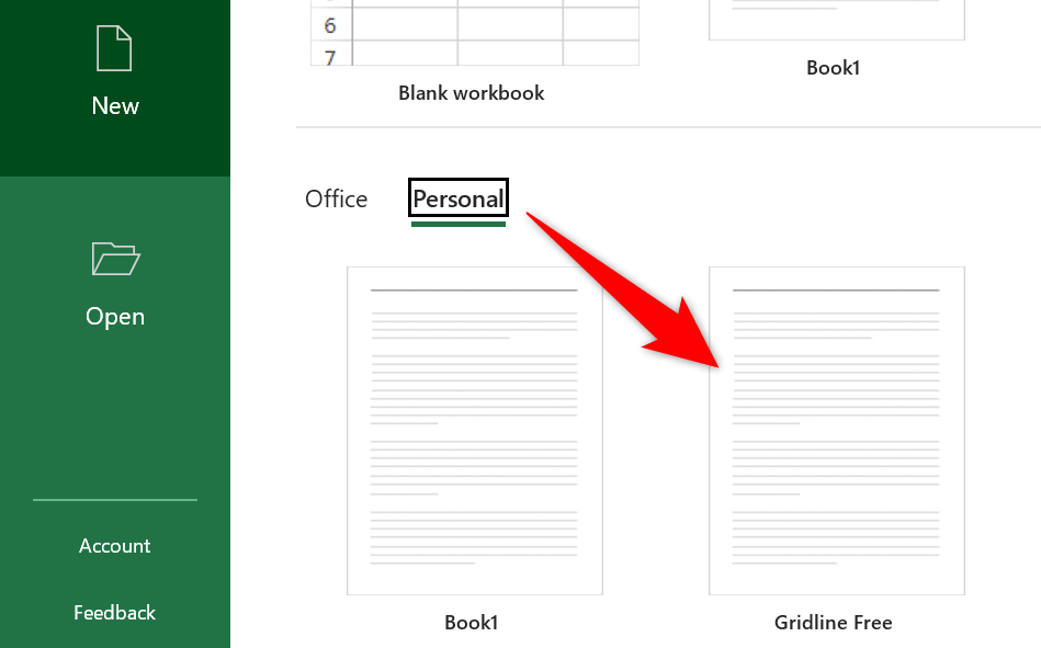
- To use this template to make spreadsheets, open Excel, select New > Personal, and select your template in the list. This will create a workbook without gridlines.
Print Gridlines in Excel
By default, gridlines aren’t printed when you print an Excel spreadsheet. If you’d like to print gridlines, enable an option in the Excel app.
- Launch your spreadsheet with Microsoft Excel.
- Select the Page Layout tab at the top of the Excel interface.
- Enable the Print option in the Gridlines section.
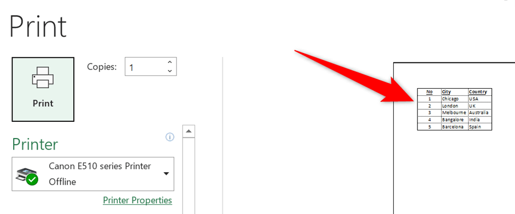
- Press Ctrl + P (Windows) or Command + P (Mac) to open the print screen. You’ll notice the print preview shows gridlines, which means your gridlines will be printed when you print your spreadsheet.
- To disable printing gridlines, turn off the Print option in the Gridlines section.
Getting Rid of Gridlines From Excel Spreadsheets
While gridlines make arranging data in your Excel spreadsheets easier, you don’t always have to use them. For the occasions when you don’t need gridlines, the methods above should help you remove gridlines from your Excel spreadsheets.


