10 Excel Tips and Tricks for 2019

In this article, I’ll be covering 10 Excel tips that you can use to boost productivity and make your work life easier. Make sure you read through the entire list so that you can find the tips that will be most useful to you.

I’ll be jumping straight into the action below. Make sure you bookmark this page so that you can come back here in case you forget any of the useful tips I’ll be sharing.

Make Use of the Status Bar

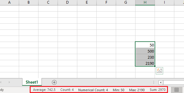
Whenever you highlight a range of numbers, the status bar at the bottom of Excel will feed you some useful information. You can find information about the sum, the average, and the total count of numbers.

Many people know about the status bar, but did you know that you can right click it to add more features? For example, you can add the minimum and maximum values in a range.

Use Shortcuts for Quick Navigation

If you need to navigate through a sheet quickly, you can use the following keyboard shortcuts.

• Ctrl+End – navigate to the furthest right cell you’ve entered data in.
• Ctrl+home – navigate to the start.
• Ctrl+right arrow – navigate to the furthest right of the Excel sheet.
• Ctrl+left arrow – navigate to the furthest left of the Excel sheet.
• Ctrl+up arrow – navigate to the top of the Excel sheet.
• Ctrl+down arrow – navigate to the bottom of the Excel sheet.

Sticky Rows

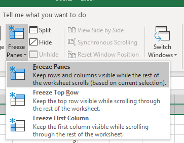
If you’d like some rows to stay at the top of the Excel sheet as you scroll through it, select the row by clicking on its letter on the left side, then click View at the top. Next, click Freeze Panes to be given the following options:

• Freeze Panes – Sticky all, based on current view.
• Freeze Top Row – Sticky only the top row.
• Freeze First Column – Stick only the first column.

Quick Select Formulas

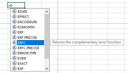
This tip can save a lot of time if you are constantly entering formulas. As you begin to type a formula, you can use the up/down arrow keys to go through suggested formulas and the tab key to automatically select that formula. This method is often much faster than typing out a formula in full each time.

Auto Fill Information

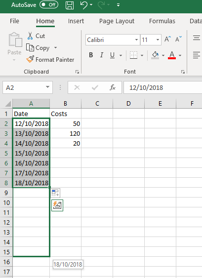
If you are filling out a range of data, you can highlight that range, then drag downward to autofill more cells with the following information. There are many ways you can use this to be more productive. For example, it can be used to automatically enter consecutive dates.

Excel is smart at guessing what information you’d like to auto fill. For example, if you have a column that shows every third day, it can follow that pattern with the auto fill feature.

Create a Macro to Automate a Task

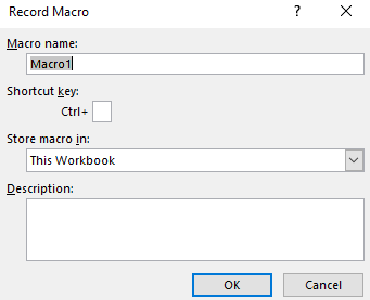
If there are any tasks you repeatedly perform in Excel, you can create a macro to automate the process. To do this, follow the steps below.

• Click File.
• Click Options.
• Click Customize Ribbon.
• Under the Main tab, select to activate the Developer box.
• Click OK.

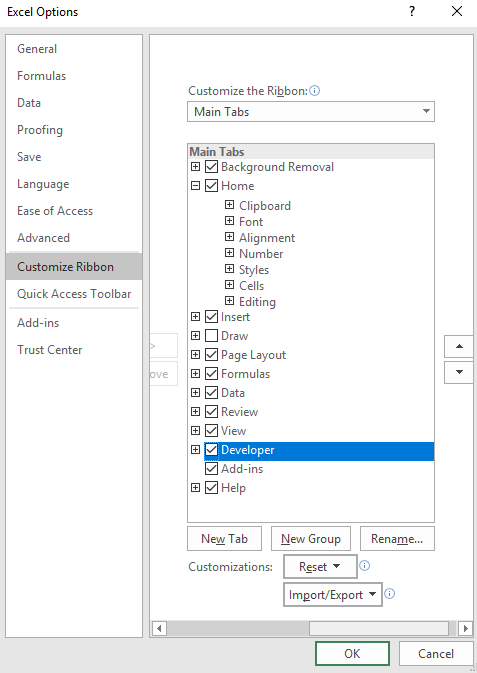
• Now, click the new Developer tab at the top of the Excel ribbon.
• After that, click the Record Macro button.
• Now, name the macro and choose a shortcut for it.
• You can also add a description to make things easier for you in the future.

• Next, simply perform any task just like you’d normally do on Excel.
• Once you’ve done, click Stop Recording.
• You can now use the shortcut you’ve created to instantly perform the task you recorded.

Create a Beautiful Table in Seconds

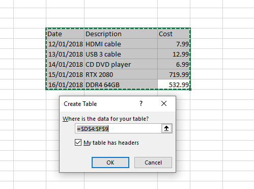
You can create visually appealing tables in seconds by following the steps below.

• First, highlight the data you’d like in the table.
• Go to the Insert tab.
• Click Table.
• The highlighted area will now have a border around it.
• Click OK to create the table.

You can use the table icons at the top right to change the colors, and use the checkboxes under the design tab to change up the layout.

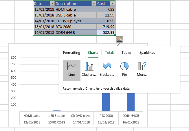
You can also click the small icon underneath the table once your cursor is hovering over the table. This will open a small menu for creating charts, tables, formatting rules, and more.

Use Go To to Find Specific Cells

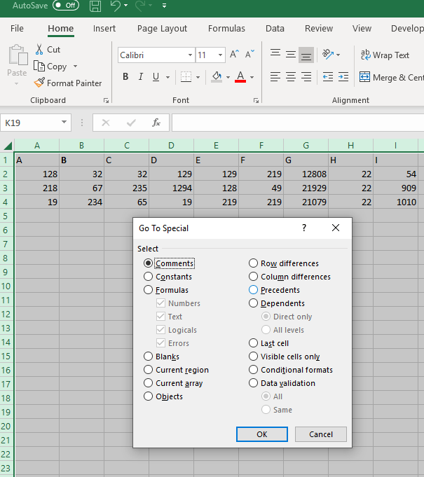
If your Excel sheet has an overwhelming amount of data, it becomes difficult to track everything down. You can use the Go To tool to find specific cells easier. It works similarly to the Find tool in Microsoft Word.

• First, select the range of data you’d like to find information in.
• Alternatively, just press Ctrl+A to select everything.
• Look for the Edit section on the Home tab at the top right.
• Click Go To.
• You can then enter a value, word, or use the ‘special’ tab to find more specific elements.

Quick tip: You can create a comment on any cells you’d like to find easily later on and then use the Comment selection in the Special tab when using Go To.

Change How ‘Enter’ Works

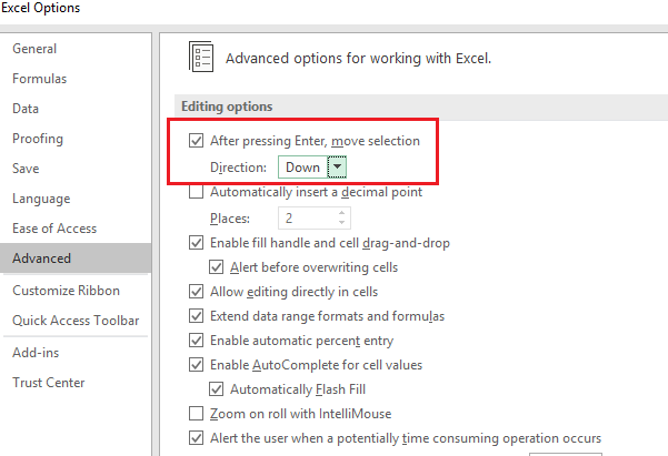
By default, pressing Enter will move you a cell down, but there is a method to change how Enter works in Excel. To change this, go to File, then Options, then click on the Advanced tab.

From here, you can choose whether the Enter key will move you up, down, right, or left. Alternatively, you can just turn off the functionality completely. This is useful if you’d like to keep enter as a simple way to confirm data and would prefer to navigate cells manually.

Copy the Same Data into Multiple Cells at Once

You can quickly copy the data of one cell into as many cells as you’d like. To do this, first press Ctrl+C on the cell you’d like to copy. Next, highlight the cells you’d like to copy to, then press Ctrl+V.

Summary

Did these Excel tips prove to be useful? I hope so. If you have any questions about the tips I’ve included in this article, please connect with me on Twitter and I’ll get back to you as soon as I can. Enjoy!