How to Calculate Annual Percentage Rate (APR) In Microsoft Excel

If you’re comparing loan offers or working out how much you’ll need to pay on your loan each year (and month), you need to find its annual percentage rate (APR). You can use Microsoft Excel to easily calculate your annual interest rate using helpful Excel formulas.

In this article, we’ll explain how to calculate the annual percentage rate in Microsoft Excel.

Table of Contents

What Is the Annual Percentage Rate?

APR is the yearly interest that’s generated by a loan you’ve taken out. APR is expressed as a percentage. This represents the extra rate that’s charged over a year, including the interest rate and additional fees (but not compounding interest).

If you take out a $100 loan with a 5% APR, you’ll pay back $105 at the end of the year — the $5 is the extra amount added by a 5% APR.

This gives you an easy way to compare different loans and helps protect you against misleading advertising.

In the US, all lenders (including credit card companies) must disclose the APR they charge to borrowers.

How to Calculate APR in Excel

APR is calculated by multiplying the loan’s periodic interest rate by the number of periods in a year. Here’s what the APR equation looks like:

Where “Interest” is the total amount of interest paid over the life of the loan, “Principal amount” is the amount of the loan, and “n” is the number of days in a loan term.

So, to calculate your APR in Excel, you need to know:

The loan amount.
The number of payment periods.
The monthly payment amount.

Then, we can use Excel to calculate the APR using various built-in functions.

Calculate Your Monthly Payment Amount

The first step is to calculate your monthly payment. If you already know this, you can skip to the next section.

If not, we’ll calculate the monthly payment using Excel’s PMT function. This is one of the financial functions, with the following formula:

=PMT(rate, nper, pv, [fv], [type])

Where:

Rate is the interest rate for the loan.
Nper is the total number of payments for the loan.
Pv is the “present value”, or the total value of the loan.
Fv is an optional quality that represents the future value of an investment or loan you want to attain after your last payment. If you leave this out, Excel will assume the future value you’re looking to attain is 0.
Type is another optional quality that explains when payments are due. The number 0 means at the start of the period, while the number 1 means at the end of the period.

To calculate PMT in Excel:

Open your Excel worksheet.
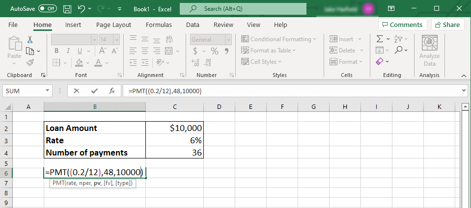
Click inside a cell and type “=PMT(rate, nper, pv)”, replacing each word with the specific values of your loan. Make sure to use the decimal value for your interest rate. So, for a 6% loan, the decimal value will be 0.06.

Press Enter and you’ll see the monthly payment amount appear.

Note: You need to keep your units consistent. If you’re calculating monthly payments, but only know the annual interest rate, make sure to divide this rate by 12 to find the monthly interest rate. Following the above example, it would be 0.06/12.

The same goes for Nper — the number of payments will be three years multiplied by 12 months, so the number of months will be 36. If you’re calculating annual payments, use the annual rate and 1 for the number of years.

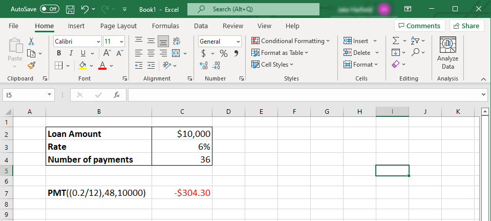
For example, imagine a $10,000 loan, on a 3-year loan (so having 36 monthly payments), with a 6% interest rate. To calculate the PMT, you would type: “=PMT((0.06/12), 36, 10000).” The resulting loan payment is: -$304.30 per month.

Excel will return a negative number when calculating the PMT. This shows that it’s money owed. If you want it to return a positive number, input the loan amount as a negative figure, instead.

Calculate the APR

With your monthly payment amount in hand, it’s time to calculate the APR. You can use this with another Excel function known as the RATE function.

The RATE function has the following format:

=RATE(nper, pmt, pv)*12

Where:

Nper is the total number of payments for the loan.
Pmt is the monthly rate calculated above.
Pv is the total value of the loan.
The final result is multiplied by 12 to get the actual annual rate, rather than monthly.

To calculate the APR in Excel:

Open your Excel workbook.
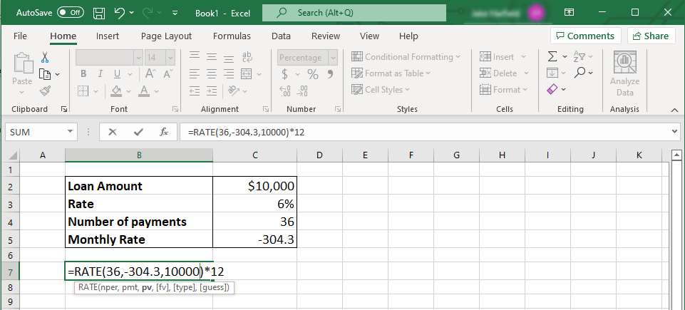
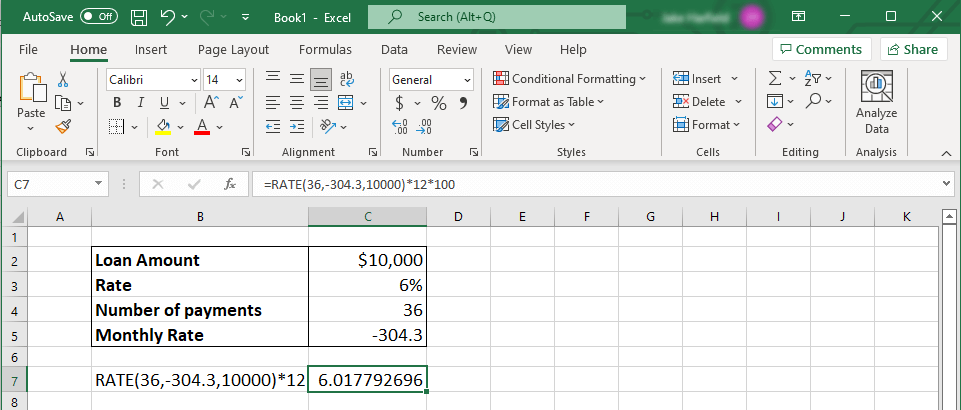
Select a cell and type: “=RATE(nper, pmt, pv)*12”, replacing each value with the quantities of your loan. The answer will be shown as a decimal value – multiply this by 100 to get the final percentage.

Press Enter.

Sticking with the example above, you’d type: “=RATE(36,-304.30,10000)*12”. The resulting APR is 6%.

Note: If you receive a #NUM! error, double-check that your syntax is correct.

Be Money Smart

Calculating the APR can help you choose the best loan and pay that loan off as quickly as possible. This is crucial if you want to make the best decisions and make your money go as far as possible.

The good thing about Microsoft Excel is that it doubles as accounting software, helping you calculate things like the annual percentage rate of your loan.